library(tidyverse)
library(colorspace)Transit Cost Analysis
Tidy Tuesday, 2021-01-05
load libraries
get the data
load the data from tidytuesdayR package
tuesdata <- tidytuesdayR::tt_load("2021-01-05")
Downloading file 1 of 1: `transit_cost.csv`raw <- tuesdata |>
pluck(1) |>
type_convert()focus
- what explains the transit costs in different continents?
- how many year the line took to build (end_year - start_year)
- length
- stations
- tunnel or ratio of tunnels from total length
- cost = real_cost / length
- add continent factor since its mentioned in the Tuesday docs
raw |> skimr::skim()| Name | raw |
| Number of rows | 544 |
| Number of columns | 20 |
| _______________________ | |
| Column type frequency: | |
| character | 11 |
| numeric | 9 |
| ________________________ | |
| Group variables | None |
Variable type: character
| skim_variable | n_missing | complete_rate | min | max | empty | n_unique | whitespace |
|---|---|---|---|---|---|---|---|
| country | 7 | 0.99 | 2 | 2 | 0 | 56 | 0 |
| city | 7 | 0.99 | 4 | 16 | 0 | 140 | 0 |
| line | 7 | 0.99 | 2 | 46 | 0 | 366 | 0 |
| start_year | 53 | 0.90 | 4 | 9 | 0 | 40 | 0 |
| end_year | 71 | 0.87 | 1 | 4 | 0 | 36 | 0 |
| tunnel_per | 32 | 0.94 | 5 | 7 | 0 | 134 | 0 |
| source1 | 12 | 0.98 | 4 | 54 | 0 | 17 | 0 |
| currency | 7 | 0.99 | 2 | 3 | 0 | 39 | 0 |
| real_cost | 0 | 1.00 | 1 | 10 | 0 | 534 | 0 |
| source2 | 10 | 0.98 | 3 | 16 | 0 | 12 | 0 |
| reference | 19 | 0.97 | 3 | 302 | 0 | 350 | 0 |
Variable type: numeric
| skim_variable | n_missing | complete_rate | mean | sd | p0 | p25 | p50 | p75 | p100 | hist |
|---|---|---|---|---|---|---|---|---|---|---|
| e | 7 | 0.99 | 7738.76 | 463.23 | 7136.00 | 7403.00 | 7705.00 | 7977.00 | 9510.00 | ▇▇▂▁▁ |
| rr | 8 | 0.99 | 0.06 | 0.24 | 0.00 | 0.00 | 0.00 | 0.00 | 1.00 | ▇▁▁▁▁ |
| length | 5 | 0.99 | 58.34 | 621.20 | 0.60 | 6.50 | 15.77 | 29.08 | 12256.98 | ▇▁▁▁▁ |
| tunnel | 32 | 0.94 | 29.38 | 344.04 | 0.00 | 3.40 | 8.91 | 21.52 | 7790.78 | ▇▁▁▁▁ |
| stations | 15 | 0.97 | 13.81 | 13.70 | 0.00 | 4.00 | 10.00 | 20.00 | 128.00 | ▇▁▁▁▁ |
| cost | 7 | 0.99 | 805438.12 | 6708033.07 | 0.00 | 2289.00 | 11000.00 | 27000.00 | 90000000.00 | ▇▁▁▁▁ |
| year | 7 | 0.99 | 2014.91 | 5.64 | 1987.00 | 2012.00 | 2016.00 | 2019.00 | 2027.00 | ▁▁▂▇▂ |
| ppp_rate | 9 | 0.98 | 0.66 | 0.87 | 0.00 | 0.24 | 0.26 | 1.00 | 5.00 | ▇▂▁▁▁ |
| cost_km_millions | 2 | 1.00 | 232.98 | 257.22 | 7.79 | 134.86 | 181.25 | 241.43 | 3928.57 | ▇▁▁▁▁ |
check quality of real_cost, start and end year column since its read as character
raw |>
  filter(if_any(c(real_cost, start_year, end_year), \(x) str_detect(x, "[[:alpha:]]", negate = TRUE)))
# A tibble: 537 × 20
e country city line start_year end_year rr length tunnel_per tunnel
<dbl> <chr> <chr> <chr> <chr> <chr> <dbl> <dbl> <chr> <dbl>
1 7136 CA Vanco… Broa… 2020 2025 0 5.7 87.72% 5
2 7137 CA Toron… Vaug… 2009 2017 0 8.6 100.00% 8.6
3 7138 CA Toron… Scar… 2020 2030 0 7.8 100.00% 7.8
4 7139 CA Toron… Onta… 2020 2030 0 15.5 57.00% 8.8
5 7144 CA Toron… Yong… 2020 2030 0 7.4 100.00% 7.4
6 7145 NL Amste… Nort… 2003 2018 0 9.7 73.00% 7.1
7 7146 CA Montr… Blue… 2020 2026 0 5.8 100.00% 5.8
8 7147 US Seatt… U-Li… 2009 2016 0 5.1 100.00% 5.1
9 7152 US Los A… Purp… 2020 2027 0 4.2 100.00% 4.2
10 7153 US Los A… Purp… 2018 2026 0 4.2 100.00% 4.2
# ℹ 527 more rows
# ℹ 10 more variables: stations <dbl>, source1 <chr>, cost <dbl>,
# currency <chr>, year <dbl>, ppp_rate <dbl>, real_cost <chr>,
# cost_km_millions <dbl>, source2 <chr>, reference <chr>eda
remove rows with missing or malformed values and convert to numeric. prepare features for analysis and modeling
transit_cost <- raw %>%
  filter(!if_any(c(start_year, end_year, real_cost), \(x) str_detect(x, "[[:alpha:]]")), real_cost != "0") |>
  type_convert() |>
  transmute(
    build_cost = real_cost / length,
    building_time_years = end_year - start_year,
    rail_lenght = length,
    how_many_stations = stations,
    tunnel_ratio = tunnel / rail_lenght,
    country = str_replace(country, "UK", "GB"),
    continent = countrycode::countrycode(country, "iso2c", "continent")
  )

transit_cost
# A tibble: 460 × 7
build_cost building_time_years rail_lenght how_many_stations tunnel_ratio
<dbl> <dbl> <dbl> <dbl> <dbl>
1 417. 5 5.7 6 0.877
2 301. 8 8.6 6 1
3 592. 10 7.8 3 1
4 465. 10 15.5 15 0.568
5 636. 10 7.4 6 1
6 415. 15 9.7 8 0.732
7 652. 6 5.8 5 1
8 344. 7 5.1 2 1
9 857. 7 4.2 2 1
10 571. 8 4.2 2 1
# ℹ 450 more rows
# ℹ 2 more variables: country <chr>, continent <chr>re-evaluate the data quality after transformation
transit_cost |> skimr::skim()| Name | transit_cost |
| Number of rows | 460 |
| Number of columns | 7 |
| _______________________ | |
| Column type frequency: | |
| character | 2 |
| numeric | 5 |
| ________________________ | |
| Group variables | None |
Variable type: character
| skim_variable | n_missing | complete_rate | min | max | empty | n_unique | whitespace |
|---|---|---|---|---|---|---|---|
| country | 0 | 1 | 2 | 2 | 0 | 56 | 0 |
| continent | 0 | 1 | 4 | 8 | 0 | 5 | 0 |
Variable type: numeric
| skim_variable | n_missing | complete_rate | mean | sd | p0 | p25 | p50 | p75 | p100 | hist |
|---|---|---|---|---|---|---|---|---|---|---|
| build_cost | 0 | 1.00 | 236.05 | 273.82 | 7.79 | 134.68 | 181.92 | 239.62 | 3928.57 | ▇▁▁▁▁ |
| building_time_years | 0 | 1.00 | 5.82 | 3.08 | 1.00 | 4.00 | 5.00 | 7.00 | 24.00 | ▇▅▁▁▁ |
| rail_lenght | 0 | 1.00 | 21.00 | 22.20 | 0.60 | 6.12 | 15.40 | 28.35 | 200.00 | ▇▁▁▁▁ |
| how_many_stations | 4 | 0.99 | 13.82 | 13.92 | 0.00 | 4.00 | 10.00 | 20.00 | 128.00 | ▇▁▁▁▁ |
| tunnel_ratio | 20 | 0.96 | 0.74 | 0.37 | 0.00 | 0.50 | 1.00 | 1.00 | 1.00 | ▂▁▁▁▇ |
how continents look like ?
africa, oceania and south america have very few datapoints, which can cause problems with modeling
transit_cost |>
  count(continent) |>
  mutate(ratio = scales::percent(n / sum(n)))
# A tibble: 5 × 3
continent n ratio
<chr> <int> <chr>
1 Africa 3 0.65%
2 Americas 36 7.83%
3 Asia 316 68.70%
4 Europe 100 21.74%
5 Oceania 5 1.09% however the data from africa, oceania and south america is not very different from other continents, so i will keep them in the analysis
transit_cost |>
    mutate(building_cost_log = log10(build_cost), .before = 1) |>
  group_by(continent) |>
  summarise(across(where(is.double), list(mean = mean, median = median)))
# A tibble: 5 × 13
continent building_cost_log_mean building_cost_log_median build_cost_mean
<chr> <dbl> <dbl> <dbl>
1 Africa 2.41 2.64 398.
2 Americas 2.59 2.50 618.
3 Asia 2.25 2.26 201.
4 Europe 2.21 2.20 193.
5 Oceania 2.55 2.55 471.
# ℹ 9 more variables: build_cost_median <dbl>, building_time_years_mean <dbl>,
# building_time_years_median <dbl>, rail_lenght_mean <dbl>,
# rail_lenght_median <dbl>, how_many_stations_mean <dbl>,
# how_many_stations_median <dbl>, tunnel_ratio_mean <dbl>,
# tunnel_ratio_median <dbl>building time per continent, the data is skewed to the right, which means that most of the lines were built in less than 10 years
transit_cost |>
  ggplot(aes(building_time_years, fill = continent)) +
  geom_histogram(binwidth = 0.8) +
  labs(
    title = "building time per continent",
    subtitle = "binwidth = 0.8"
  )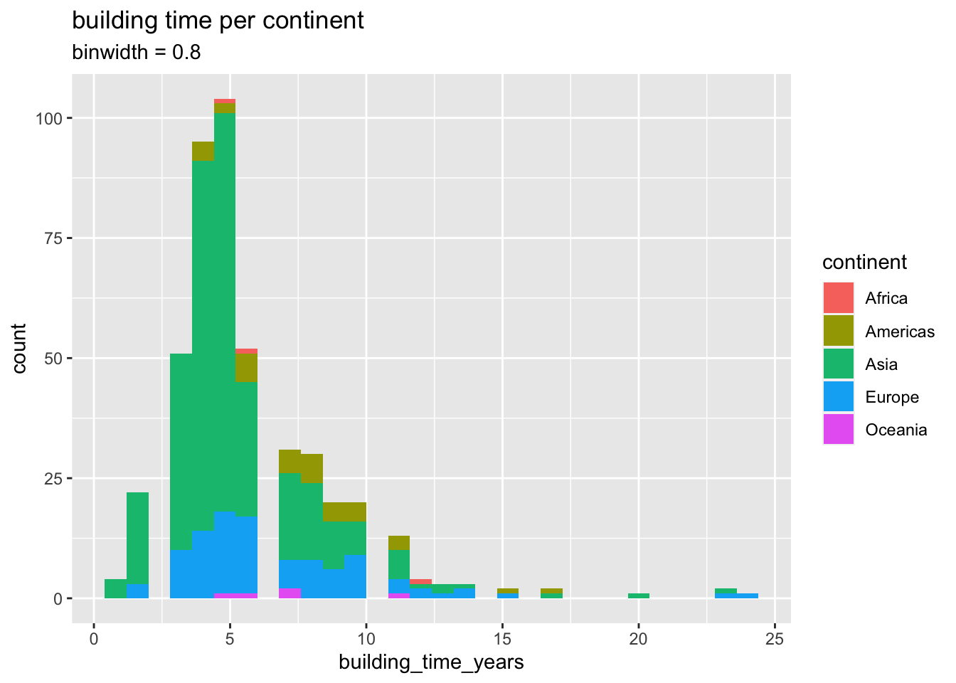
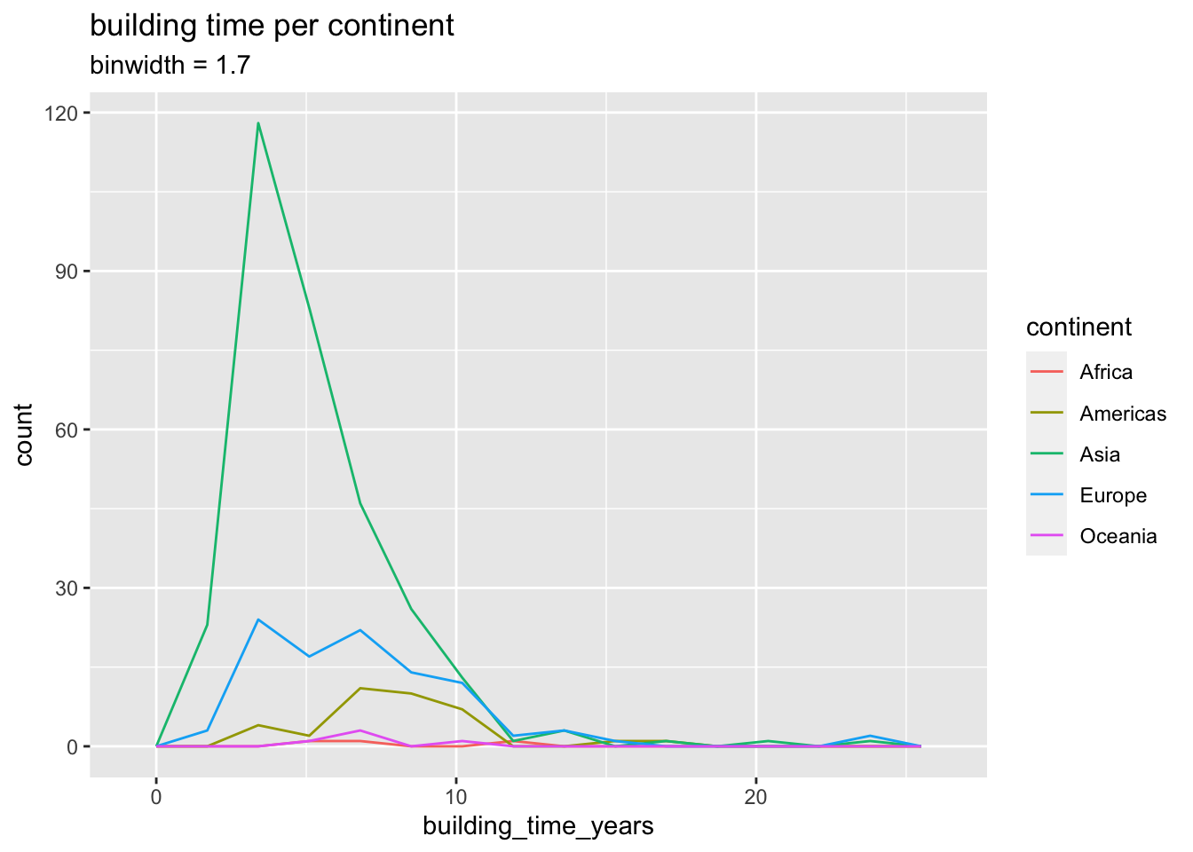
this represent the building time better, asia seems to build the lines faster than other continents. however if track lenght is taken into account, the picture changes.
b_size <- 1.7
transit_cost |>
  ggplot(aes(building_time_years)) +
  geom_freqpoly(aes(color = continent), binwidth = b_size) +
  labs(
    title = "building time per continent",
    subtitle = str_glue("binwidth = {b_size}")
  )
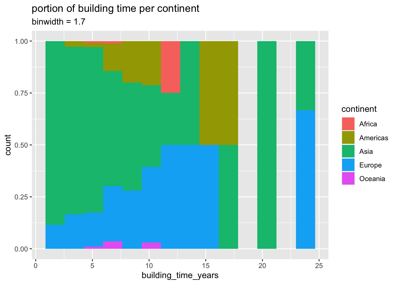
transit_cost |>
  ggplot(aes(building_time_years)) +
  geom_histogram(aes(fill = continent), position = "fill", binwidth = b_size) +
  labs(
    title = "portion of building time per continent",
    subtitle = str_glue("binwidth = {b_size}")
  )
building time vs track lenght
# scatter plot with building time and track lenght
transit_cost |>
  ggplot(aes(building_time_years, rail_lenght, color = continent)) +
  geom_jitter(alpha = 1 / 2) +
  geom_smooth(method = "lm", se = F) +
  labs(title = "building time vs track lenght",
       subtitle = "y scale is per continent") +
  theme(legend.position = "bottom") +
  scale_color_discrete_sequential(palette = "Heat") +
  facet_wrap(vars(continent), scales = "free_y")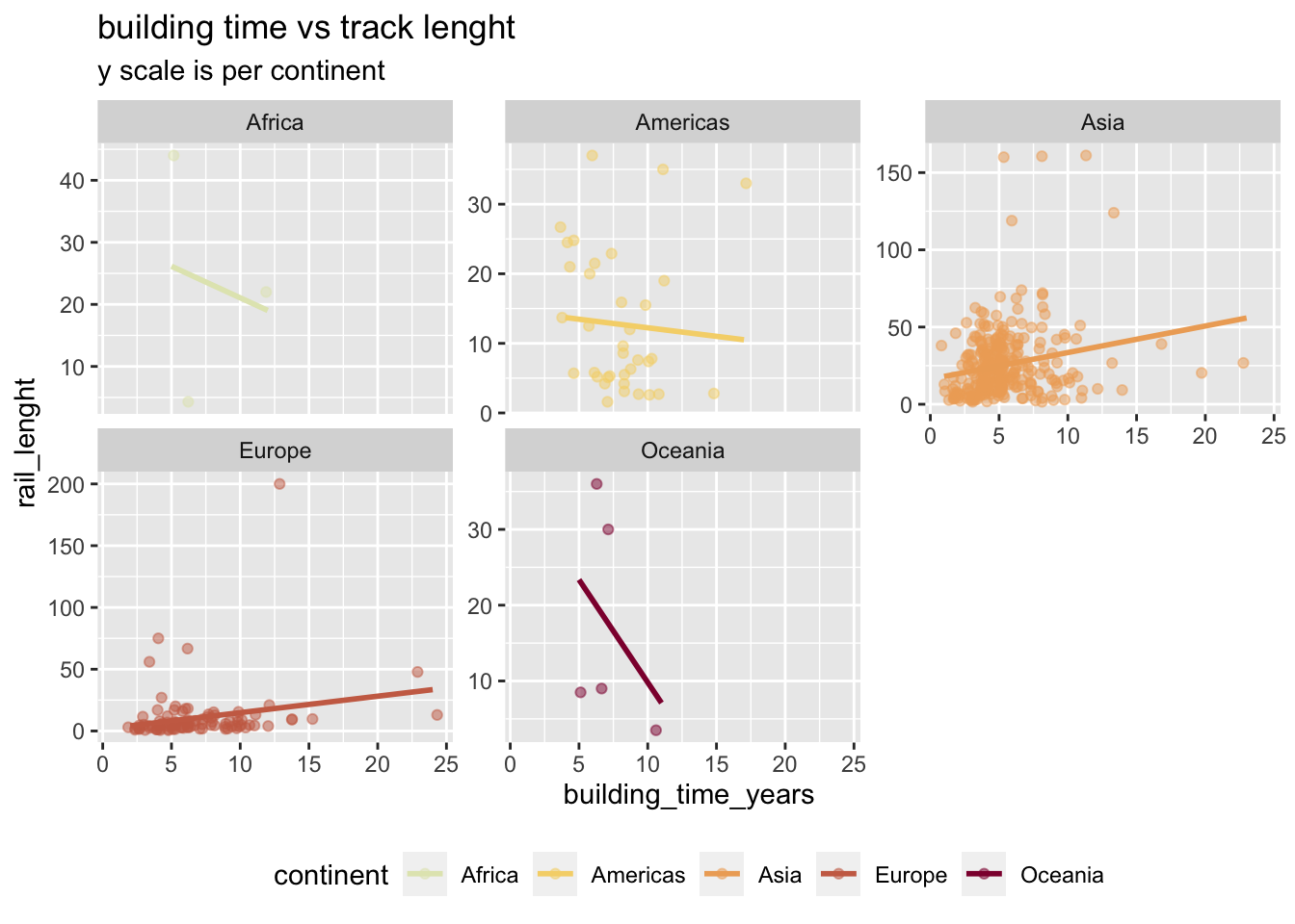
correlation
complete dataset
tunnel ratio and building time have statistically significant correlation to build cost. correlation against build cost is not very strong, but it is statistically significant.
library(correlation)
transit_cost |>
  correlation() |>
  summary()
# Correlation Matrix (pearson-method)
Parameter | tunnel_ratio | how_many_stations | rail_lenght | building_time_years
------------------------------------------------------------------------------------------
build_cost | 0.16** | -0.10 | -0.10 | 0.24***
building_time_years | -0.03 | 0.13* | 0.10 |
rail_lenght | -0.21*** | 0.85*** | |
how_many_stations | -0.24*** | | |
p-value adjustment method: Holm (1979)per continent
correlation in continents is not strong.
transit_cost |>
  group_by(continent) |>
  correlation() |>
  summary()
# Correlation Matrix (pearson-method)
Group | Parameter | tunnel_ratio | how_many_stations | rail_lenght | building_time_years
-----------------------------------------------------------------------------------------------------
Africa | build_cost | 0.95 | -0.99 | -1.00 | 0.25
Africa | building_time_years | -0.05 | -0.13 | -0.19 |
Africa | rail_lenght | -0.97 | 1.00 | |
Africa | how_many_stations | -0.98 | | |
Americas | build_cost | 0.32 | -0.45* | -0.48* | 0.40
Americas | building_time_years | 0.09 | -0.02 | -0.07 |
Americas | rail_lenght | -0.42 | 0.90*** | |
Americas | how_many_stations | -0.39 | | |
Asia | build_cost | 0.19** | 0.03 | 9.58e-03 | 0.15*
Asia | building_time_years | -0.17* | 0.22*** | 0.21** |
Asia | rail_lenght | -0.13 | 0.85*** | |
Asia | how_many_stations | -0.18* | | |
Europe | build_cost | 0.24 | -0.04 | 1.67e-03 | 0.23
Europe | building_time_years | 0.10 | 0.36** | 0.22 |
Europe | rail_lenght | -0.14 | 0.87*** | |
Europe | how_many_stations | -0.09 | | |
Oceania | build_cost | 0.58 | -0.45 | -0.63 | 0.77
Oceania | building_time_years | 0.30 | -0.26 | -0.42 |
Oceania | rail_lenght | -0.99* | 0.89 | |
Oceania | how_many_stations | -0.88 | | |
p-value adjustment method: Holm (1979)modeling
library(tidymodels)
tidymodels_prefer()
split data to training and testing, i dont use validation set since the data size is small testing set purpose is to confirm that the build model has potential to work with new data. i use log10 of build cost to make the data more normal distributed.
set.seed(123)

transit_cost_log <- transit_cost |>
  mutate(build_cost = log10(build_cost))

split <- initial_split(transit_cost_log, prop = 0.8)
trn <- training(split)
tst <- testing(split)
recipe
building tune and tunnel ratio seemed to have correlation with building cost. some of the tunnel ratios were missing, i use mean imputation to insert replacement data. i also add recipe with all features to see if it improves the model.
transit_rec <- recipe(build_cost ~ building_time_years + tunnel_ratio, data = trn) %>%
  step_impute_mean(tunnel_ratio) |>
  prep()
cross validation
I am using standard 10 fold cross validation to test the models later. cross validation is used to estimate how well the model will perform in practice without using the test set.
transit_folds <- vfold_cv(trn, v = 10)
transit_folds
# 10-fold cross-validation
# A tibble: 10 × 2
splits id
<list> <chr>
1 <split [331/37]> Fold01
2 <split [331/37]> Fold02
3 <split [331/37]> Fold03
4 <split [331/37]> Fold04
5 <split [331/37]> Fold05
6 <split [331/37]> Fold06
7 <split [331/37]> Fold07
8 <split [331/37]> Fold08
9 <split [332/36]> Fold09
10 <split [332/36]> Fold10select models
low bias (blackbox) models can learn the relationship so well that it memorizes the training set, which means that when model is used with test data, the performance can degrade. linear regression is the most simple model, but it can be used as a baseline to compare other models. random forest and xgboost are blackbox models, which can learn complex relationships, but they are prone to overfitting. cross validation can help to reduce overfitting.
models <- list(lin = linear_reg(), rand = rand_forest(mode = "regression"), xg = boost_tree(mode = "regression"))
modelset <- workflow_set(list(transit_rec), models)
keep_pred <- control_resamples(save_pred = TRUE, save_workflow = TRUE)
metrics_list <- metric_set(rmse, rsq, mae)
fit models
workflowmap has all the models and recipes in a list and it fits all the models to the training set.
fit_models <- function(.data) {
  .data |>
    workflow_map("fit_resamples",
      seed = 10101, verbose = T,
      resamples = transit_folds, control = keep_pred,
      metrics = metrics_list
    )
}

res <- modelset |> fit_models()

res
# A workflow set/tibble: 3 × 4
wflow_id info option result
<chr> <list> <list> <list>
1 recipe_lin <tibble [1 × 4]> <opts[3]> <rsmp[+]>
2 recipe_rand <tibble [1 × 4]> <opts[3]> <rsmp[+]>
3 recipe_xg <tibble [1 × 4]> <opts[3]> <rsmp[+]>evaluate models
rmse is used to evaluate the models, since it is easy to interpret and it is in the same units as the target variable. based on ranking, linear regression is the best model based on rmse. however the difference between the models is not very big.
res |> collect_metrics()# A tibble: 9 × 9
wflow_id .config preproc model .metric .estimator mean n std_err
<chr> <chr> <chr> <chr> <chr> <chr> <dbl> <int> <dbl>
1 recipe_lin Preprocesso… recipe line… mae standard 0.187 10 0.0111
2 recipe_lin Preprocesso… recipe line… rmse standard 0.265 10 0.0188
3 recipe_lin Preprocesso… recipe line… rsq standard 0.142 10 0.0412
4 recipe_rand Preprocesso… recipe rand… mae standard 0.196 10 0.0100
5 recipe_rand Preprocesso… recipe rand… rmse standard 0.272 10 0.0156
6 recipe_rand Preprocesso… recipe rand… rsq standard 0.102 10 0.0258
7 recipe_xg Preprocesso… recipe boos… mae standard 0.205 10 0.0118
8 recipe_xg Preprocesso… recipe boos… rmse standard 0.285 10 0.0176
9 recipe_xg Preprocesso… recipe boos… rsq standard 0.0839 10 0.0172res |> autoplot()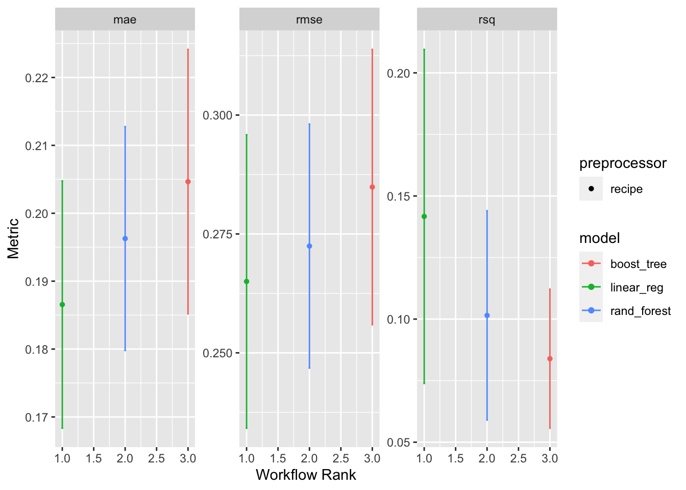
res |> rank_results(rank_metric = "rmse")# A tibble: 9 × 9
wflow_id .config .metric mean std_err n preprocessor model rank
<chr> <chr> <chr> <dbl> <dbl> <int> <chr> <chr> <int>
1 recipe_lin Preprocesso… mae 0.187 0.0111 10 recipe line… 1
2 recipe_lin Preprocesso… rmse 0.265 0.0188 10 recipe line… 1
3 recipe_lin Preprocesso… rsq 0.142 0.0412 10 recipe line… 1
4 recipe_rand Preprocesso… mae 0.196 0.0100 10 recipe rand… 2
5 recipe_rand Preprocesso… rmse 0.272 0.0156 10 recipe rand… 2
6 recipe_rand Preprocesso… rsq 0.102 0.0258 10 recipe rand… 2
7 recipe_xg Preprocesso… mae 0.205 0.0118 10 recipe boos… 3
8 recipe_xg Preprocesso… rmse 0.285 0.0176 10 recipe boos… 3
9 recipe_xg Preprocesso… rsq 0.0839 0.0172 10 recipe boos… 3tune hyperparameters
lets tune the hyperparameters of random forest and xgboost models to see if we can improve the performance. I will keep the linear regression model as a baseline.
xg_tune <- boost_tree(
  mode = "regression",
  trees = 1000,
  min_n = tune(),
  tree_depth = tune(),
  learn_rate = tune()
)
xg_tune
Boosted Tree Model Specification (regression)
Main Arguments:
trees = 1000
min_n = tune()
tree_depth = tune()
learn_rate = tune()
Computational engine: xgboost rf_tune <- rand_forest(
mode = "regression",
mtry = tune(),
trees = 1000,
min_n = tune()
)
modelset2 <- workflow_set(list(pari = transit_rec), list(reg = linear_reg(),rf_tune = rf_tune, xg_tune = xg_tune), cross = TRUE)
modelset2# A workflow set/tibble: 3 × 4
wflow_id info option result
<chr> <list> <list> <list>
1 pari_reg <tibble [1 × 4]> <opts[0]> <list [0]>
2 pari_rf_tune <tibble [1 × 4]> <opts[0]> <list [0]>
3 pari_xg_tune <tibble [1 × 4]> <opts[0]> <list [0]>res2 <- modelset2 |> workflow_map(
resamples = transit_folds, grid = 10, verbose = TRUE, seed = 10102,
control = keep_pred,
metrics = metrics_list
)
res2 |> collect_metrics() |>
arrange(-mean)# A tibble: 63 × 9
wflow_id .config preproc model .metric .estimator mean n std_err
<chr> <chr> <chr> <chr> <chr> <chr> <dbl> <int> <dbl>
1 pari_xg_tune Preprocess… recipe boos… rmse standard 0.576 10 0.0206
2 pari_xg_tune Preprocess… recipe boos… mae standard 0.523 10 0.0195
3 pari_xg_tune Preprocess… recipe boos… rmse standard 0.308 10 0.0171
4 pari_xg_tune Preprocess… recipe boos… rmse standard 0.298 10 0.0168
5 pari_xg_tune Preprocess… recipe boos… rmse standard 0.295 10 0.0160
6 pari_xg_tune Preprocess… recipe boos… rmse standard 0.287 10 0.0165
7 pari_xg_tune Preprocess… recipe boos… rmse standard 0.286 10 0.0162
8 pari_rf_tune Preprocess… recipe rand… rmse standard 0.284 10 0.0153
9 pari_rf_tune Preprocess… recipe rand… rmse standard 0.283 10 0.0153
10 pari_rf_tune Preprocess… recipe rand… rmse standard 0.279 10 0.0150
# ℹ 53 more rowsanalyse models
generally there is little diffence between the models, this is due to dataset being simple (small amount of features and datapoints), whic means simple liner regression can learn the relationship well. Below its clear that non tuned models are quite simeilar to tuned models.
library(patchwork)
 res |> autoplot() / res2 |> autoplot() + plot_annotation(title = "Non Tuned (top row) vs Tuned models (bottom row)")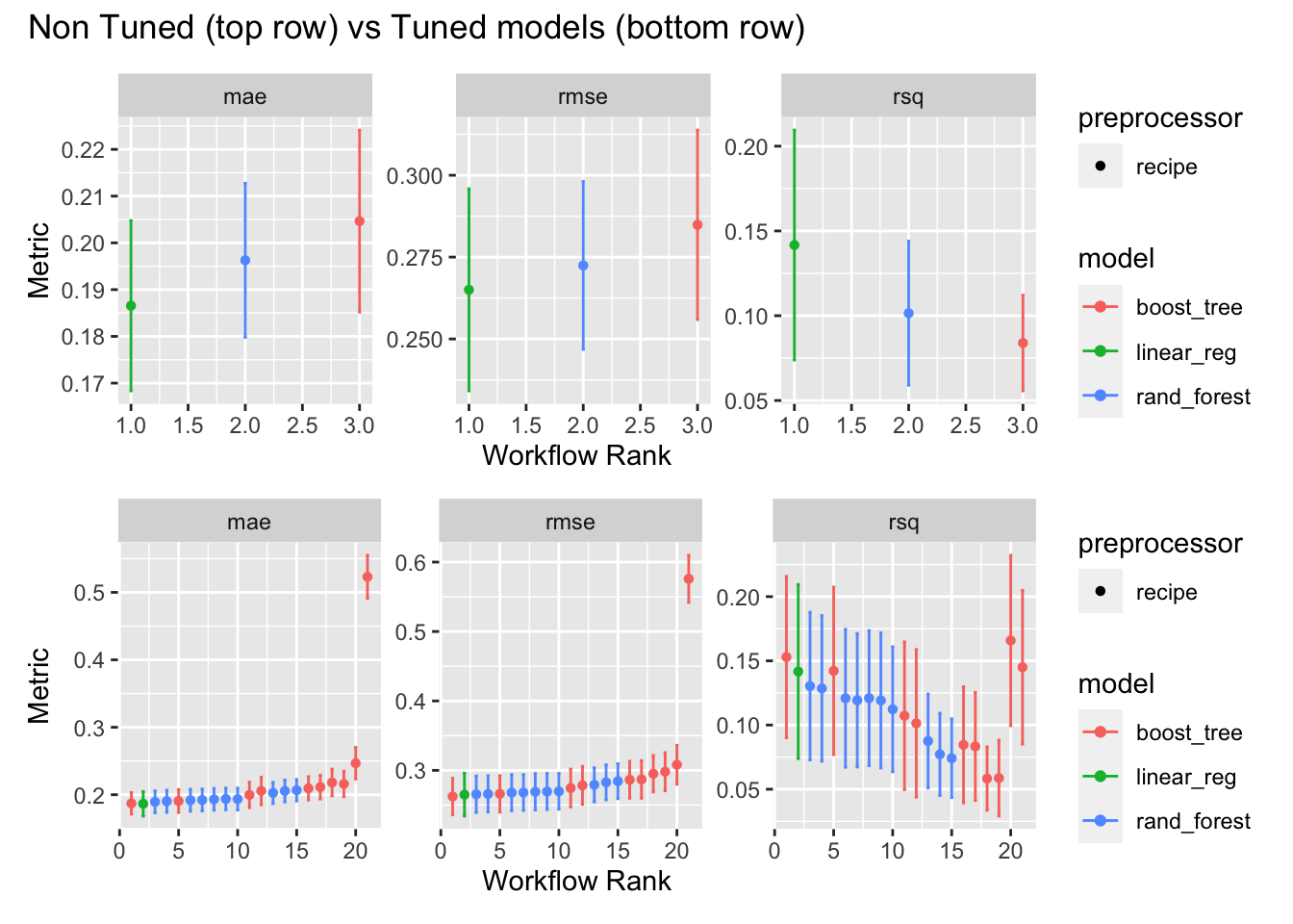
select model
select best model based on rmse metric and fit to the whole training set
bestmodel <- res2 |>
  extract_workflow_set_result("pari_xg_tune") |>
  select_best(metric = "rmse")
bestmodel
# A tibble: 1 × 4
min_n tree_depth learn_rate .config
<int> <int> <dbl> <chr>
1 33 1 0.0539 Preprocessor1_Model08result <- res2 |>
extract_workflow("pari_xg_tune") |>
finalize_workflow(bestmodel) |>
last_fit(split = split)the modeling is done, but out of curiosity lets if there is a difference between training metrics and test metrics. rmse is slightly higher in test set, but the difference is not big, which means that the model is not overfitting.
result |>
  collect_predictions() |>
  metrics(truth = build_cost, estimate = .pred)
# A tibble: 3 × 3
.metric .estimator .estimate
<chr> <chr> <dbl>
1 rmse standard 0.227
2 rsq standard 0.0733
3 mae standard 0.178 rank_results(res2, rank_metric = "rmse", select_best = TRUE) # A tibble: 9 × 9
wflow_id .config .metric mean std_err n preprocessor model rank
<chr> <chr> <chr> <dbl> <dbl> <int> <chr> <chr> <int>
1 pari_xg_tune Preprocesso… mae 0.187 0.00972 10 recipe boos… 1
2 pari_xg_tune Preprocesso… rmse 0.262 0.0160 10 recipe boos… 1
3 pari_xg_tune Preprocesso… rsq 0.153 0.0382 10 recipe boos… 1
4 pari_reg Preprocesso… mae 0.187 0.0111 10 recipe line… 2
5 pari_reg Preprocesso… rmse 0.265 0.0188 10 recipe line… 2
6 pari_reg Preprocesso… rsq 0.142 0.0412 10 recipe line… 2
7 pari_rf_tune Preprocesso… mae 0.189 0.00993 10 recipe rand… 3
8 pari_rf_tune Preprocesso… rmse 0.266 0.0160 10 recipe rand… 3
9 pari_rf_tune Preprocesso… rsq 0.130 0.0350 10 recipe rand… 3check predicions vs actual values
Plot the predictions vs actual values. I convert the values back to original scale to make the plot more readable for human. Generally the predictions are close to actual values, but there are some outliers.
result |>
  collect_predictions() |>
    mutate(build_cost = 10 ^ build_cost,
           .pred = 10^.pred) |>
  ggplot(aes(.pred, build_cost)) +
  geom_point(alpha = 0.5) +
  geom_abline() +
  coord_obs_pred() +
  labs(title = "Predicted vs actual value") +
  labs(x = "Predicted", y = "Actual")
transit_cost |>
    summarise(build_cost = mean(build_cost), #add other statistical metrics
              sd = sd(build_cost),
              median = median(build_cost),
              min = min(build_cost),
              max = max(build_cost),
              n = n())
# A tibble: 1 × 6
build_cost sd median min max n
<dbl> <dbl> <dbl> <dbl> <dbl> <int>
1 236. NA 236. 236. 236. 460